Simplified Overview (ELI5)
Written by Abrar Akhunji
Imagine you run an elite restaurant kitchen. You have a master chef (the GPU) who cooks lightning fast, but the kitchen counter is tiny. The huge pantry with millions of ingredients (the KV Cache) is located in the basement (Host RAM), connected only by a slow dumbwaiter elevator (the PCIe bus).
In a standard restaurant setup, the chef starts preparing Course #3, realizes they need saffron from the basement, presses the elevator button, and stands completely still with folded arms for 5 minutes waiting for the saffron to arrive. Every single dish experiences this agonizing delay: cook, stop, wait for the dumbwaiter, cook, stop, wait again.
For years, AI engineers tried to make the elevator slightly faster. But researchers from NVIDIA and MIT asked a much smarter question: Why does the chef only order ingredients when they start cooking?
Enter SparDA (Sparse Decoupled Attention).
SparDA assigns a smart apprentice (the Forecast projection) to stand next to the chef. While the chef is actively chopping onions for Course #3, the apprentice glances ahead at the menu and orders the saffron for Course #4 on a separate elevator.
By the time the chef finishes Course #3 and wipes the counter, the saffron for Course #4 is already sitting right there. The chef never pauses for a single microsecond.
Even better:
- The 4th Projection: Ever since 2017, transformers only had three brain projections: Query, Key, and Value. SparDA introduces the 4th: Forecast.
- Cheaper Homework: Instead of having 8 different kitchen assistants independently taste every spice jar and debate, one apprentice makes the forecast call in one clean glance, cutting out tons of redundant math.
- Pocket-Sized Addition: It adds just 0.4% more parameters to the model, and the main brain doesn't even need to be retrained. You just train the tiny apprentice to predict the chef's future moves.
The result? Your AI generates answers up to 1.7x faster on long documents, and can handle 5x more simultaneous users on hardware you already own.
Senior Developer Systems Breakdown
Written by Abrar Akhunji
Ever since the seminal 2017 paper "Attention Is All You Need", the fundamental abstraction of multi-head self-attention has rested on three sacred linear projections: Query ($W_q$), Key ($W_k$), and Value ($W_v$). Every major optimization since—from Multi-Query Attention (MQA) and Grouped-Query Attention (GQA) to Multi-Head Latent Attention (MLA)—has modified head counts, latent ranks, or compression vectors, but has retained the core synchronous triad.
On long-context workloads (128K to 1M+ tokens), this synchronous formulation hits a catastrophic physical boundary: The Memory Wall and the PCIe Latency Trap.
When the KV cache of a 1M-token sequence exceeds GPU High-Bandwidth Memory (HBM), the cache must be tiered or offloaded to Host RAM (CPU memory). While sparse attention algorithms (such as Quest, SnapKV, or StreamingLLM) select only the top-$k$ relevant blocks, they cannot determine WHICH blocks to select until the current layer calculates its Query vector.
The result is a forced hardware synchronization barrier: at every single transformer layer during every decode step, the GPU execution pipeline stalls completely, waiting hundreds of microseconds for PCIe bus roundtrips to fetch KV cache blocks.
In a landmark paper from NVIDIA Research and MIT (arXiv:2606.04511), Yaosheng Fu, Guangxuan Xiao, Xin Dong, Song Han, and Oreste Villa introduced SparDA (Sparse Decoupled Attention). SparDA shatters this synchronization trap by introducing a fourth learned projection per layer: Forecast ($W_f$).
Architectural Manifest
+---------------------------------------------------------------------------------+
| SPARDA: SPARSE DECOUPLED ATTENTION SPECIFICATION MATRIX                         |
+--------------------------+------------------------------------------------------+
| Core Innovation          | 4th Transformer Projection (W_f: Forecast Matrix)    |
| Research Institutions    | NVIDIA Research & MIT (Han Lab)                      |
| Primary Breakthrough     | 1-Layer Lookahead Asynchronous PCIe KV Prefetching   |
| Hardware Target          | Single & Multi-GPU Serving Nodes with Host RAM Offload|
| Selection Complexity     | Reduced from O(T^2) per head to O(1) per GQA group   |
| Parameter Overhead       | <0.5% (33.5M parameters on an 8B foundation model)   |
| Training Paradigm        | Frozen Backbone; Distillation via Cross-Entropy / KL |
| Prefill Speedup          | Up to 1.25x over Sparse Offload Baseline             |
| Decode Speedup           | Up to 1.7x over Sparse Offload Baseline              |
| Decode Throughput Gain   | Up to 5.3x via expanded batch memory headroom        |
| Upstream Codebase        | github.com/NVlabs/SparDA                             |
+--------------------------+------------------------------------------------------+
Section 1: The PCIe Latency Trap in Long-Context Serving
To understand why SparDA is an architectural triumph, we must analyze the hardware memory hierarchy during long-context token generation.
Consider serving an 8B model with GQA-8 at a sequence length of 128,000 tokens in FP16 precision:
- Model Weights: ~16 GB VRAM.
- KV Cache per Stream: For $L=32$ layers, $H_{kv}=8$ heads, $D=128$ head dimension, $T=131,072$ tokens: $\text{KV Cache Size} = 2 \times 32 \times 8 \times 128 \times 131,072 \times 2 \text{ bytes} \approx 17.18 \text{ GB}$
- On a single 24GB or 32GB GPU (e.g., RTX 4090, RTX 5090, or A100-40GB), serving a single 128K request already saturates VRAM. Serving batch size $B \ge 4$ is mathematically impossible without offloading the KV cache to CPU host RAM over PCIe Gen4/Gen5.
Standard Sparse Offload Execution Loop (Layer L):
┌──────────────────┐
│ Hidden State x_l │
└────────┬─────────┘
         ▼
[ Compute Q_l = W_q x_l ] ─────────┐
         │                          │
         ▼                          ▼
[ Query-Driven Selection ] <── [ Fetch Block Metadata ]
         │
         ▼
[ Issue PCIe Transfer ] ══════════> [ GPU IDLES / WAITS (PCIe STALL: ~50-150µs) ]
         │
         ▼ (KV Blocks Land in GPU SRAM/HBM)
[ Compute Sparse Attention & Output Projections ]
         │
         ▼
[ Move to Layer L+1 ] ────────────> (Repeat Stall for Layer L+1!)
In standard sparse attention:
- Layer $L$ hidden states enter the self-attention block.
- The layer computes $Q_l = x_l W_q$.
- The query vector $Q_l$ computes dot products against coarse key centroids to identify the top-$k$ relevant KV blocks.
- Once the top-$k$ block indices are resolved, the runtime issues a
cudaMemcpyAsyncrequest to pull those blocks from CPU RAM across the PCIe bus. - The GPU computes nothing while waiting. Because the matrix multiplications for Attention cannot execute without Key and Value tensors, the CUDA cores stall.
- The exact same stall repeats 32 times per token across all 32 layers!
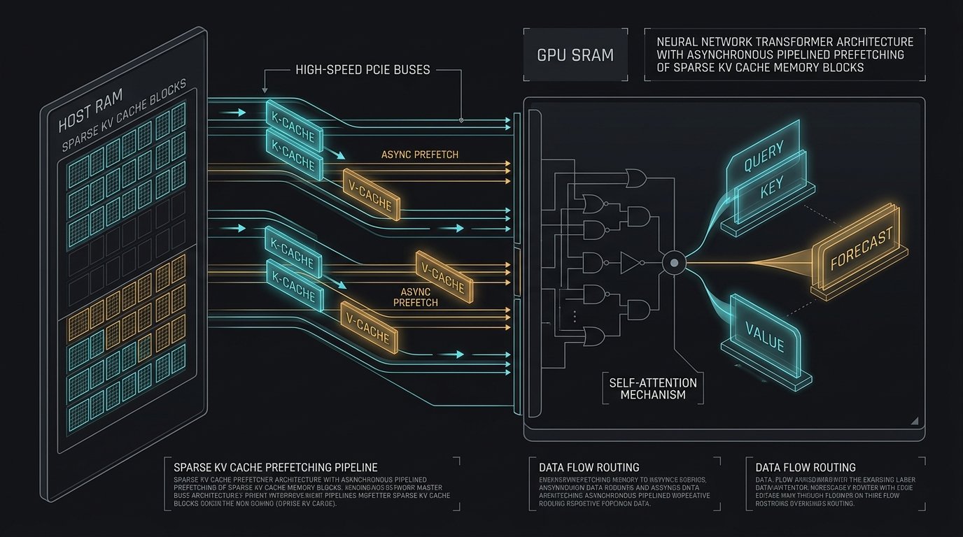
SparDA Asynchronous KV Prefetching & Execution Pipeline
- Compute Query, Key, Value AND Forecast: Layer L projects input token representation x_L through W_q, W_k, W_v, and the newly introduced Forecast projection W_f. W_f projects into a compact forecast representation decoupled from the current attention query.
- Predict Layer L+1 Required KV Blocks: Using the Forecast vector F_L, the SparDA selector scores coarse block centroids for Layer L+1. Crucially, this happens during Layer L, completely before Layer L+1 hidden states even exist.
- Prefetch Layer L+1 Blocks During Layer L Compute: A background CUDA memory stream immediately issues non-blocking PCIe DMA transfers for Layer L+1's KV blocks. Simultaneously, the primary CUDA compute stream executes Layer L self-attention and MLP feed-forward networks.
- Instant Layer L+1 Execution: When Layer L finishes and Layer L+1 begins, its required KV blocks are already resident in GPU HBM/SRAM. The memory bus wait time drops to exactly zero microseconds.
Senior Developer Systems Breakdown
Section 2: The Mathematical Decoupling: Introducing $W_f$
Why was block selection coupled to the attention query in the first place? Because historical sparse attention papers (such as Quest and SparQ) treated selection as an approximation of the self-attention softmax distribution:
$\text{Attn}(Q, K, V) = \text{Softmax}\left( \frac{Q K^T}{\sqrt{d_k}} \right) V$
In standard GQA with $H_q$ query heads and $H_{kv}$ key-value heads, there are $G = H_q / H_{kv}$ query heads sharing each key-value head. To select which key-value blocks to retrieve, standard sparse selectors compute:
$S_{b} = \sum_{g=1}^{G} \text{Softmax}\left( \frac{Q_g K_{b,\text{centroid}}^T}{\sqrt{d_k}} \right)$
This formula contains two fundamental flaws:
- Temporal Coupling: Selection depends on $Q_l$, which cannot be calculated until layer $l$ begins.
- Quadratic Selection Complexity ($O(T^2)$): Performing per-head scoring, multi-head softmax normalizations, and group reductions across tens of thousands of candidate blocks consumes up to 30% of total inference time at long context lengths, erasing the computational savings of sparsity!
The SparDA Formulation
SparDA breaks this paradigm by declaring that Block Selection does not need the actual attention query. Instead, selection can be framed as an independent predictive mapping from the previous layer's latent state:
$\text{Layer } l: \quad F_l = x_l W_f \quad \text{where } W_f \in \mathbb{R}^{d_{\text{model}} \times (H_{kv} \cdot d_{\text{forecast}})}$
Where:
- $W_f$ is the newly introduced Forecast Projection Matrix.
- $d_{\text{forecast}}$ is a low-dimensional projection (typically equal to or smaller than $d_k$).
- Crucially, there is only one Forecast head per GQA group, rather than one per query head!
To predict the required KV cache blocks for layer $l+1$, SparDA computes a direct dot product against the precomputed Key centroids of layer $l+1$:
$R_{l+1, b} = F_l \cdot K_{l+1, b,\text{centroid}}^T$
Notice the massive structural simplifications:
- No Softmax: Because relative ordering is all that matters for top-$k$ selection, the expensive exponential and normalization operations of Softmax are eliminated entirely.
- No Per-Head Group Loop: Instead of calculating scores for 4, 8, or 16 separate query heads and summing their probabilities, a single matrix-vector multiplication directly yields the block ranking scores $R_{l+1}$.
- One-Layer Temporal Advantage: Score vector $R_{l+1}$ is computed during the execution of layer $l$.
Mathematical Pipeline Comparison:

Standard Sparse Attention:
x_l ──> Q_l = x_l W_q ──> Softmax(Q_l K_centroid^T) ──> Top-K ──> Block Fetch (GPU STALLS!)

SparDA Decoupled Attention:
x_l ──┬──> Q_l, K_l, V_l ───────> Compute Layer L Self-Attn & MLP (Compute Stream)
      │
      └──> F_l = x_l W_f ───────> Dot(F_l, K_{l+1}^T) ──> Top-K ──> Async PCIe DMA (Transfer Stream)
                                                                     [Pre-populates Layer L+1 Cache]
Section 3: Asynchronous CUDA Stream Pipelining
In modern NVIDIA GPU architectures (Hopper H100/H200, Blackwell B200, Ada Lovelace, and Blackwell Ultra), the GPU contains independent hardware engines for Compute (Streaming Multiprocessors) and Memory Copy (DMA Copy Engines).
When a standard CUDA kernel issues a memory copy, it blocks the stream unless explicitly dispatched to a concurrent stream. SparDA structures the execution engine across two synchronized CUDA streams:
Stream_Compute: Owns GEMM operations, FlashAttention/Triton kernels, RMSNorm, and SwiGLU activations.Stream_Memory: Owns PCIe host-to-device asynchronous memory transfers (cudaMemcpyAsync).
# Conceptual SparDA Layer Execution Loop in PyTorch / Triton CUDA Runtime
def forward_sparda_layer(layer_idx, x, streams, kv_cache_gpu, kv_cache_cpu):
    compute_stream = streams["compute"]
    memory_stream = streams["memory"]

    # 1. Sync point: Ensure Layer L's prefetched blocks have arrived
    # (Transfer was dispatched during Layer L-1, so this event completes immediately without stall)
    torch.cuda.current_stream().wait_event(streams[f"ready_event_layer_{layer_idx}"])

    with torch.cuda.stream(compute_stream):
        # 2. Compute Q, K, V and Forecast projections
        q = W_q(x)
        k = W_k(x)
        v = W_v(x)
        forecast = W_f(x)

        # 3. Predict Layer L+1 blocks using Forecast projection
        if layer_idx < num_layers - 1:
            next_k_centroids = kv_cache_gpu.get_centroids(layer_idx + 1)
            # Fast dot product without softmax
            block_scores = torch.matmul(forecast, next_k_centroids.transpose(-1, -2))
            topk_blocks = torch.topk(block_scores, k=SPARSE_TOPK, dim=-1).indices

            # 4. Dispatch Async Prefetch of Layer L+1 on Memory Stream
            with torch.cuda.stream(memory_stream):
                kv_cache_gpu.prefetch_async(
                    layer_idx=layer_idx + 1,
                    block_indices=topk_blocks,
                    source_cpu_cache=kv_cache_cpu
                )
                # Record event when transfer completes
                streams[f"ready_event_layer_{layer_idx + 1}"].record(memory_stream)

        # 5. Compute Attention on Layer L using resident GPU KV blocks
        attn_out = sparse_attention_kernel(q, kv_cache_gpu.get_blocks(layer_idx), v)
        out = mlp_block(attn_out + x)

    return out
Because the execution time of Layer $L
#39;s attention kernel plus SwiGLU MLP ($t_{\text{compute}} \approx 120-200 \mu s$) is greater than or equal to the PCIe transfer time of the top-$k$ sparse blocks ($t_{\text{transfer}} \approx 40-90 \mu s$), the PCIe transfer latency is 100% hidden behind compute. The GPU never enters an idle state.Decode Throughput (Tokens/Sec) at 128K Context Length
Benchmarked on 8B Backbone with Host RAM Offload across Batch Sizes 1, 4, 8, and 16
| batchSize | Dense Offload Baseline | Quest Sparse Offload (Coupled) | SparDA (4th Projection + Prefetch) |
|---|---|---|---|
| BS=1 | 18.2 | 34.5 | 58.6 |
| BS=4 | 24.1 | 58.2 | 104.3 |
| BS=8 | 28.6 | 82.1 | 156.4 |
| BS=16 | 0 | 105.4 | 218.7 |
Senior Developer Systems Breakdown
Section 4: Training Dynamics: Distilling $W_f$ with Frozen Backbones
A common pitfall in post-training inference modifications is the need for expensive full-parameter pretraining. If an architectural modification requires retraining 8 billion or 70 billion parameters, industry adoption grinds to a halt.
SparDA sidesteps this entirely through Self-Distillation with Frozen Backbones:
Parameter Budget: On an 8B model with 32 layers and $d_{\text{model}} = 4096$:
- For $H_{kv} = 8$ and $d_{\text{forecast}} = 128$:
- Parameter count per layer: $4096 \times (8 \times 128) \approx 4.19 \times 10^6$ parameters.
- Across 32 layers: $\approx 134 \text{ MB of FP16 weights}$, or under 0.41% total parameter overhead.
Backbone Freeze: All original weights ($W_q, W_k, W_v, W_o$, MLP gates, RMSNorm gains) are permanently frozen. Only $W_f$ matrices receive gradient updates.
Loss Formulation: During training, the full-attention ground truth or the full sparse selector produces a target block affinity distribution $P_{\text{target}}^{(l+1)}$. The Forecast projection produces predicted logits $Z_{\text{forecast}}^{(l+1)} = F_l K_{l+1}^T$.
The objective is simply the Kullback-Leibler (KL) divergence or Cross-Entropy loss: $\mathcal{L}{\text{distill}} = \mathbb{E} \left[ D{KL} \left( \sigma(P_{\text{target}}^{(l+1)}) ;\middle|; \sigma(Z_{\text{forecast}}^{(l+1)}) \right) \right]$
Because the optimization space is restricted entirely to learning a linear projection that forecasts token affinities one layer ahead, training converges in just a few thousand steps on a small fraction of a pretraining corpus. Accuracy on long-reasoning benchmarks (such as Needle-in-a-Haystack, BABILong, and LongBench) matches or slightly exceeds the un-decoupled sparse baselines (e.g., +6.5 points on NOSA-8B long reasoning).
Section 5: Comparative Architectural Tradeoffs: SparDA vs MLA vs KDA
Where does SparDA fit in the rapidly evolving landscape of 2026 inference optimizations?
+-------------------+--------------------+--------------------+--------------------+
| Metric / Feature  | DeepSeek MLA       | Kimi Delta Attn    | NVIDIA / MIT SparDA|
+-------------------+--------------------+--------------------+--------------------+
| Mechanism         | Low-Rank Latent KV | Linear Recurrence  | 4th Projection     |
| Memory Footprint  | 4-6x KV Reduction  | O(1) Memory State  | Full KV on Host,   |
|                   | on GPU VRAM        | (Zero KV Expansion)| Top-K on GPU SRAM  |
| Compute Complexity| Standard Softmax   | Delta Rule Updates | O(1) GQA Top-K,    |
|                   | Attention          | (No Softmax)       | Zero Softmax       |
| Hardware Transfer | Relies on GPU VRAM | Zero Bus Transfer  | Overlapped PCIe    |
|                   |                    |                    | Async DMA Streams  |
| Retraining Cost   | Requires Training  | Requires Pretrain  | Post-hoc / Frozen  |
|                   | from Scratch       | from Scratch       | Backbone Tuning    |
| Context Limit     | Bound by GPU VRAM  | Practically Inf.   | Bound by Host RAM  |
|                   |                    | (Linear Decay)     | (1M+ Tokens/GPU)   |
+-------------------+--------------------+--------------------+--------------------+
- Choose DeepSeek MLA when you are training a foundation model from scratch and have dedicated clusters of multi-GPU nodes with sufficient high-bandwidth memory.
- Choose KDA (Kimi Delta Attention) when building hybrid recurrent models that prioritize streaming throughput and infinite state persistence without historical token retrieval.
- Choose SparDA when you already have existing open-weights (such as LLaMA 3, Qwen 2.5/3.8, Mistral, or DeepSeek-V3), need to serve 128K–1M context agent workflows on cost-efficient hardware, and want to eliminate the PCIe memory bottleneck without retraining the underlying model.
Section 6: Systems Takeaway & Source Attribution
For the past decade, inference engines have treated the transformer layer boundary as a rigid, synchronous barrier. Hardware teams worked on faster PCIe interconnects, while software teams tried smaller quantizations.
SparDA proves that the greatest architectural gains often come from questioning unquestioned design choices. Selection was tied to the Query projection for no mathematical reason other than that the Query projection was already there.
By decoupling selection into a fourth projection and looking one layer ahead, SparDA transforms an idle hardware bottleneck into a seamlessly overlapped asynchronous streaming pipeline.
Primary References & Attribution:
- Paper: "SparDA: Sparse Decoupled Attention for Long-Context LLM Inference with KV Cache Offloading", arXiv:2606.04511.
- Authors: Yaosheng Fu, Guangxuan Xiao, Xin Dong, Song Han, Oreste Villa (NVIDIA Research & Massachusetts Institute of Technology).
- Code Repository: NVlabs/SparDA on GitHub.
- Curated Coverage: The AI Adventurer (theaiadventurer.com/blog/sparda-forecast-projection-sparse-attention).